• Thesis to Book with ISBN
• Aim And Scope
• Article in Press
• Editorial Board
• Current Issue
• Archives
• Publication Charges
• Authors Information
• Contact Us
• Paper Format

 [Abstract] [PDF] [HTML] [Linked References]

On Half-Cauchy Distribution and Process

Elsamma  Jacob¹  , K Jayakumar²

¹Malabar Christian College, Calicut, Kerala, INDIA.

²Department of Statistics, University of Calicut, Kerala, INDIA.

Corresponding Address:

[email protected], [email protected]

Research Article

Abstract: A new form of half- Cauchy distribution using Marshall-Olkin transformation is introduced. The properties of the new distribution such as density, cumulative distribution function, quantiles, measure of skewness and distribution of the extremes are obtained. Time series models with half-Cauchy distribution as stationary marginal distributions are not developed so far.  We develop   first order autoregressive process with the new distribution as stationary marginal distribution and the properties of the process are studied. Application of the distribution in various fields is also discussed.

Keywords:  Autoregressive Process, Geometric Extreme Stable, Half-Cauchy Distribution, Skewness, Stationarity, Quantiles.

1. Introduction:

The  half  Cauchy (HC) distribution is  derived  from  the  standard  Cauchy distribution  by  folding  the  curve  on  the  origin  so  that  only  positive  values can  be  observed.  A continuous random variable X is said to have the half Cauchy distribution if its survival function is given by

As  a  heavy  tailed  distribution,  the  HC  distribution  has  been  used  as  an alternative  to  exponential  distribution  to  model  dispersal  distances  (Shaw
(1995)) as the former predicts more frequent long distance dispersed events than  the  latter.   Paradis  et.al  (2002)  used  the  HC  distribution  to  model ringing data on two species of tits (Parus caeruleus and Parus major) in
Britain and Ireland.

From (1.1), we get the probability density function (pdf )  f (x) and cumulative distribution function (cdf ) F(x) of the HC distribution as 

and

respectively, see Johnson et al.  (2004). The Laplace transform of (1.2) is

where

Remark 1.1.  For the HC distribution the moments do not exist.

Relationship with other distributions:

1. Let Y be a folded t variable with pdf given by

When  , (1.5)   reduces to

Thus, HC distribution coincides with the folded t distribution with degree of freedom.

2.  Let Z₁ and Z₂ be two independent non negative, real valued rvs having the folded standard normal distribution.   Then   has the HC distribution.

3.  It is known that the folded standard normal distribution coincides with the chi-square distribution with one degree of freedom.  Therefore, if Z₁ and Z₂ are two independent chi-square variables with parameter 1, then  has the HC distribution.

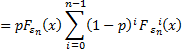
According to Gaver and Lewis (1980), a self decomposable distribution can be the marginal distribution of a stationary   first order autoregressive (AR(1)) process of the form

Where { is a sequence of independent identically distributed (i.i.d) random variables, independent of Xn.  The usual procedure to develop AR(1) models of  the  form  (1.6)  for  self  decomposable  distributions  is  by  considering  the generating functions.  Here since the Laplace transform of HC distribution is not in closed form, we use the minification model introduced by Pillai et al. (1995) to develop first order autoregressive process with HC distribution as stationary marginal distribution.

Adding  parameters  to  an  existing  distribution  will  give  extended  forms of  the  distribution  and  these  distributions  are  more  flexible  to  model  real data.  Marshall and Olkin (1997) introduced a general method of adding a parameter to a family of distributions. According to them, if F(x) denote the cdf of a continuous rv X , then

is also  a  proper  cdf.  In  this  paper,  we  introduce  a  new  family  of  HC  distribution by applying transformation (1.7) to the HC distribution and using
this new class, we develop an autoregressive maximum process with the new form  of  HC  distribution  as  stationary  marginal  distribution  and  study  its
properties.

The paper is organized as follows:  The generalized half Cauchy distribution is introduced and some of its properties are given in section 2.  Section 3
deals with the estimation of the parameter.  First order autoregressive process with the new distribution as stationary marginal distribution is introduced
and its properties are studied in section 4.  Simulated sample path behavior of the process and autoregressive process of order k are given in this section.
Section 5 gives the concluding remarks and the possible area of application of the new model.

2. Generalized Half-Cauchy Distribution:

A generalization of the HC distribution, named Beta Half-Cauchy distribution obtained through beta transformation was introduced by Cordeiro and Lemonte (2011).  Here,  we  introduce  another  generalization  of  the  HC  distribution, which  has  simple  closed  form  expression  for  the  cdf,  using  the Marshall-Olkin transformation.  By substituting the cdf (1.3) in transformation (1.7), we get a new family of HC distribution with cdf

When  , (2.1) reduces to  (1.3).  The pdf is obtained as

and the survival function is

We  call  the  distribution  with  cdf  given  by  (2.1)  as  the  Generalized  half-Cauchy distribution with parameter  denoted as GHC().

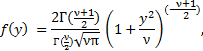
Fig.1 pdf of GHC( ) for   = 2, 1:5, 1, 0.8, 0.2, 0.5

The hazard rate function is

(2.3)

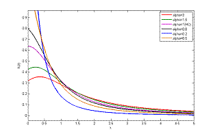
Fig.2 hazard rate function of GHC() for  = 2, 1,5, 1, 0.8, 0.5, 0.3, 0.2

The shapes of the density function for various values of the parameter are given in   figure 1.  Figure 2 shows the shapes of the hazard rate function for  selected  values  of  The  new  model  is  very  simple  and  can  be  easily simulated as follows. If U is an Uniform (0,1) random variable, then   has GHC() distribution.

Remark  2.1.  The  mode  of  the  distribution  is  the  solution  of  the  equation

Remark 2.2.  For the GHC() distribution the moments do not exist. (Theorem 1 Rubio and Steel (2012)) .

The q^th  quantile of the GHC() distribution  is given by

 where 0

and (.) is the inverse distribution function. For
 the median and quartiles are respectively

The quartile measure of skewness is obtained as

Definition  2.3  (Marshall  and  Olkin  (1997)).   Let     be a sequence of independent identically distributed random variables with common cdf  F (x)  and  let  N  be  a  geometric  random  variable  with  parameter  p  such that P (N  = n) = p(1-p) ^n-1 , n=1,2,….; 0<p<1, which is independent of X_i  for all  Also, let U=min(X₁,X₂,,,,, X_N) and V = max(X₁,X₂,,,,, X_N).  If  implies  that  the  distribution  of  U (V )  is  in  ,  then    is said  to  be  geometric-minimum  stable  (geometric-maximum  stable).  If    is both  geometric-minimum  and  geometric-maximum  stable,  then   is  said  to be geometric-extreme stable.

Theorem  2.4.  Let   and  N  are defined as  in  definition  (2.3). Then,

(i)  min(X₁,X₂,,,,, X_N) has GHC() distribution,

(ii)  max(X₁,X₂,,,,, X_N) has GHC  distribution.

Proof.  Let  U = min(X₁,X₂, …. X_N) and V=max(X₁,X₂,X_N). The survival function of U  is given by

P (U   x) =  P(min(X₁,X₂,,,,, X_N)    x)

                  = 

                  =

That is, GHC() distribution is geometric minimum stable.  Similarly, the cdf of V  is given by

P (V   x) =  P(max(X₁,X₂,,,,, X_N)   x)

                  = 

                  = ,

which shows that the distribution is geometric maximum stable.

Remark 2.5. It follows from definition (2.3) and theorem (2.4) that GHC() distribution is geometric extreme stable.

3. Estimation of Parameters:

The log-likelihood of the sample is given by

Log L =  nlog(2 

2

The normal equation is

The maximum likelihood estimate of     is the solution of equation (3.1).  It can be solved numerically by using the function nlm in the statistical software R.

4. First order AR process with GHC() as marginal distribution:

In this section, we develop stationary autoregressive maximum process with GHC() marginal distribution.  The autoregressive sequence {X_n} of GHC()distributed random variables are related in the following manner:

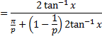
where  0  <  p  <  1  and  {  is  a  sequence  of  i.i.d  HC  random  variables, independent of {X_n}.

Theorem 4.1.  {X_n} as defined by (4.1) is a stationary AR(1) process with GHC (1/p)  marginal  distribution  if  and  only  if  {  is  distributed  as  HC, provided              (1/p).

Proof. From (4.1),

assuming stationarity.  Let   with cdf (1.3). Then,

 =

Conversely, Let  (1/p)

=  

    =

To prove stationarity, let (1/p) and X₁ is as defined by (4.1).

Now, let  (1/p) and X_n   is as defined by (4.1). Following similar steps, it can be shown that  (1/p).  Hence the proof.

Remark 4.2.  Even if X₀ is distributed arbitrary with cdf , the process is asymptotically stationary with (1/p) marginal distribution.

Proof.  Let X₀ is distributed arbitrary with cdf and   Using the autoregressive structure (4.1), the cdf of Xn can be expressed as

as n  and since 0 < p < 1.

Now, if H is obtained as

Hence X_n converges in distribution to GH C (1/p) as               n .

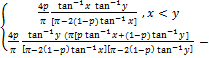
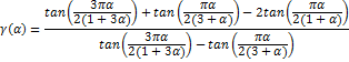
Now  we  consider  the  joint  distribution  of  the  random  variables  X_n  and X_n-1 . We have

The joint distribution of the random variables X_n and X_n-1 is not absolutely continuous since

On the other hand, we have that

(a)

(b)

(c)

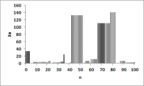
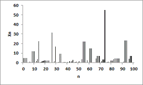
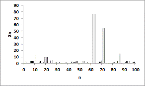
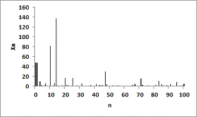
(d)

fig. 3 Simulated Sample path of the Process GHC()

The simulated sample path for the GHC() process for   = 0.1, 0.3, 0.6, 0.9 is given in figure 3, (a) – (d).  The inferences can be verified by referring to the expression for P (X_n < X_n-1).

The introduced maximum autoregressive process of the   first order can be easily generalized to high-order process.  Namely, we can introduce maximum autoregressive process of order k as following

Where 0  p_i < 1 for i = 0,1,….,k and .  Then, {X_n} is a stationary process with GHC (1/p₀) marginal distribution if and only if {} is distributed as HC.  We have that

On assuming stationarity, we get

Thus,  (1/). This shows that the first order model can be easily extended to the k^th order case and all results derived above are valid here also.

5. Conclusion

In this paper, we use the transformation introduced by Marshall and Olkin (1997)  to  define  a  new  model  called  Generalized  half-Cauchy  distribution, which  extends  the  half-Cauchy  distribution.   We  study  some  properties  of the model and discuss the maximum likelihood estimation of its parameters. The  proposed  model  is  more   flexible  than  the  half-Cauchy  distribution  and can be used effectively for modeling lifetime data. First order autoregressive process with half-Cauchy distribution as stationary marginal distribution is developed for the first time and the properties of the process are studied.

References: