 |
||||||
|
|
Home| Journals | Statistics Online Expert | About Us | Contact Us | |||||
 |
||||||
| About this Journal | Table of Contents | ||||||
|
|
[Abstract]
[PDF]
[HTML]
[Linked
References] A Stochastic Analysis of Two Competitive Interacting Species with Bionomic Harvesting of Both the Species
R. Srilatha1*, B. Ravindra Reddy2†, N. Ch. Pattabhiramacharyulu3 1Sree Chaitanya Inst. of Tech. & Sci., Thimmapur, Karimnagar-505527, Andhra Pradesh, INDIA. 2Department of Mathematics, JNTUH CE, Nachupally, Karimnagar-505501, Andhra Pradesh, INDIA. 3Professor (Retd.) of Mathematics, NIT, Warangal – 506004, Andhra Pradesh, INDIA. Corresponding Addresses: *[email protected], †[email protected] Research Article
Abstract: This paper deals with two species competitive model with both the first and second species are harvested under bionomic conditions. The model is characterized by a pair of first order non-linear ordinary differential equations. All the possible equilibrium points of the model are identified and the criteria for the local and global stabilities are discussed .The possibility of existence of bio economic equilibrium is being discussed. We also provide analytical estimates of the population intensities of fluctuations by Fourier transform methods.
There is an extensive study on several kinds of prey- predator interactions after it was initiated by Lotka [1] and Volterra [2]. Bionomics of natural resources has played a significant role in all these interactions. There is a strong impact of harvesting on the dynamic evolution of a population. In fishery, forestry, agriculture and wild life management, the exploitation of biological resources and harvesting of population species can be seen. The problems of predator-prey systems in the presence of harvesting were discussed by many authors and attention on economic policies from harvesting have also been analysed. A detailed discussion on the issues and techniques associated with the bionomic exploitation of natural resources was given by Clark [3, 4]. A study on a class of predator-prey models under constant rate of harvesting of both species simultaneously was made by Brauer and Soudack [5, 6]. Multi-species harvesting models are also studied in detail by Chaudhuri [7, 8]. In the study of population dynamics, many Mathematical models have been proposed. In order to reflect the dynamical behavior of the models depending on the existing data and information of the system, it is often necessary to incorporate stochastic term with additive noise. For long time, it has been recognized that stochastic terms have very complicated impact on the dynamics of a system, which can not cause the instability but also induce some noise, in terms of oscillations and periodic solutions. Models on the combined harvesting of a two species prey predator fishery have been discussed by Ragozin and Brown [9], Chaudhuri and Saha Ray [11], etc. A resource based competitive system in three species with persistence and global stability of the system was studied by chattopadhyaya and et.al. [10]. Prey-predator model with harvesting was also studied by Dai and Tang [12]. In 1973, Holling [15] emphasized the influence of noise in ecological dynamics and resilience. The noise may arise from stochastic disturbance of the external environment. Under the disturbance of noise, the species dynamics are always stochastic or seemingly stochastic. In 1996 J. Ripa et. al [16] examined the noise colour and the risk of population extinction in a prey predator system widely. In 2003 Xu, C, et.al [14] investigated about White noise or noise with a white variance spectrum contains no temporal autocorrelation and is essentially a series of independent random numbers about the population dynamics and color environmental noise of a three species food chain system. Later in 2009, Sun, G.Q et.al [17] emphasized the role of noise in a predator–prey model with Allee effect. In 2011, Wenting Wang et.al [18] found the effect of colored noise on spatiotemporal dynamics of biological invasion in a diffusive predator-prey system. K. Shiva Reddy et.al [13] proposed the mathematical model for the three species ecosystem comprising of two predators competing for the prey. They also investigated the stability concepts using various mathematical techniques. In this connection here we constructed a mathematical model based on the system of non-linear equations. The global stability of the system at interior steady state is determined and illustrated numerically. The conditions of the existence of a bionomic equilibrium are discussed by taking simple economic considerations into an account. We also provide analytical estimates of the population intensities of fluctuations by Fourier transform methods.2. Mathematical Model The model equations for a two species competitive system are given by the following system of non-linear ordinary differential equations
where
3. Analysis of Equilibrium Points The steady state equations of (2.1)-(2.2) are
Case (i): The population is extinct and this steady state always exists. Case (ii): If which is always positive because of the initial assumption Case (iii): If Case (iv): If
4. Discussion about Local Stability In this section the characteristic equation is
Since the sum of the roots of (4.1) is which is negative and the product of the roots is positive, the roots of (4.1) can be noted to be negative. Hence the system is locally asymptotically stable.
5. Discussion about Global Stability Theorem: The Equilibrium point Proof: let us consider the following Liapunov function
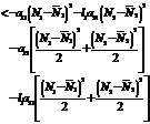
where Differentiating V w.r.to‘t’ we get
<0 Hence6. Bionomic Equilibrium The bionomic equilibrium is nothing but the combination of the concepts of biological equilibrium as well as economic equilibrium. A biological equilibrium is given by Where
In order to determine the bionomic equilibrium we come across the following cases. Case (i): If for the second species, fishing cost is greater than the revenue (
Case (ii): If the cost is greater than the revenue in the first species fishing, then the first species fishing will be closed (i.e.
(6.5) Case (iii): If Case (iv): If In this case Substitute (6.6) and (6.7) in (6.1), (6.2) we get
7. A Stochastic Model The main assumption that leads us to extend the deterministic model (2.1)-(2.2) to a stochastic counterpart is that it is reasonable to conceive the open sea as a noisy environment. There are many number of ways in which environmental noise may be incorporated in system (2.1)-(2.2). Note that environmental noise should be distinguished from demographic or internal noise, for which the variation over time is due. External noise may arise either form random fluctuations of one or more model parameters around some known mean values or from stochastic fluctuations of the population densities around some constant values. In this section, we compute the population intensities of fluctuations (variances) around the positive equilibrium
where
where Let
Using (7.3), equation (7.1) becomes
The linear part of (7.4) is
Again using (7.3) equation (7.2) becomes
+ The linear part of (7.6) is Taking the Fourier transform on both sides of (7.5), (7.7) we get,
The matrix form of (7.8),(7.9) is
where
Eqn.(7.10) can also be written as Let where if the function where
If
The corresponding variance of fluctuations in
and the auto correlation function is the normalized auto covariance
For a Gaussian white noise process, it is
From (7.12), we have From (7.14) we have
Hence by (7.16) and (7.20), the intensities of fluctuations in the variable
and by (7.13), we obtain
where Real part of Imaginary part of Finally from (7.11) we get
By substitution of (7.23), (7.11) in (7.22), we get,
If we are interested in the dynamics of system (7.1)-(7.2) with either If
If
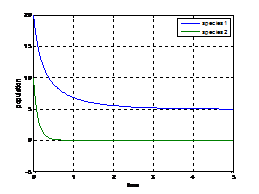
8. Numerical Simulation In this paper, we substantiate as well as augment our analytical findings through numerical simulations considering the following parameters. Example (1):
Figure (8.1) Figure (8.1) shows that the variation of population against time, initially with
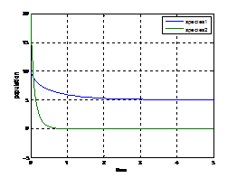
Example(2):
Figure (8.2) Figure (8.2) shows that the variation of population against time initially with9. Discussion and Concluding Remarks In this paper, a model of a competitive system with stochastic term was formulated. Initially we have discussed about the model without stochastic term and investigated the existence of equilibrium points, local stability by employing Routh-Hurwitz criteria, global stability by constructing Lyapunov function. We incorporated the stochastic term in the model, also we present spatial competition model that contains some important factors, and such as the population intensities of fluctuations (variances) around the positive equilibrium due to noise are computed and also analyzed the stability with graphical representation using Matlab. Some Numerical simulations for justifying the theoretical analysis are also provided. Here we studied about the competitive model by incorporating environmental fluctuations through additive White noise. The analytical results and numerical simulation of deterministic model suggest that the deterministic competitive model is stable. The stable nature of the system shows this situation in figures (8.1)-(8.2). Further for stochastic model system population vacancies characterize the stochastic stability of the system. Therefore by contolling the environmental fluctuations, the existence of the system can be checked.
References
|
|||||
|
||||||


