|
|
||||||
|
|
Home| Journals | Statistics Online Expert | About Us | Contact Us | |||||
 |
||||||
| About this Journal | Table of Contents | ||||||
|
|
[Abstract] [PDF] [HTML] [Linked References]
Multi-Objective Inventory Model of Deteriorating Items with Shortages in Fuzzy Environment
Omprakash Jadhav1, V.H. Bajaj2 Department of Statistics, Dr. B. A. M. University, Aurangabad, Maharashtra-431004, INDIA.
Abstract: In this paper multi-objective inventory model under limited storage area, deteriorating. Items with stock-dependent demand are developed in a fuzzy environment. Here, objectives are to maximize the profit and to minimize the total average cost and wastage cost, where Purchasing price, set-up cost, holding cost, storage area, Inventory cost, shortage cost, rate of deterioration, total storage area, and objective goals are fuzzy in nature. In this model, fuzzy parameters are represented by linear membership functions and after the fuzzification, it is solved by fuzzy non-linear programming (FNLP) and weight FNLP (WFNLP), fuzzy product goal programming, (FPGP) and weight FPGP (WFPGP) method are presented. The model is illustrated numerically and the results obtained from both WFNLP and WFPGP methods. Solving this problem also for some numerical values by both WFNLP and WFPGP methods, optimum results are presented in tabular form for different weights. Key words: Multi- objective, Deteriorating items, Shortages, Fuzzy Goal Programming, Linear membership functions.
1. Introduction Though Multi-Objective Decision Making (MODM) problems have been formulated in many areas like air pollution, transportation, structural analysis etc. It may depend on time, on hand inventory level or initial stock level, etc. After that, the models with time dependent demand rate have been studied by several researchers Datta and pal [6], Chen and Wang [5], Bakhi [1] and others. In this area, a lot of research papers have been published by several researches such as Papachristos and Skouri [8], Chang et. al. [3], Balkhi [1], Chang [4] and others. However, Goyal and Giri [7] presented a review article on deteriorating items including the publications up to 2001.Over the past two decades, no extensive research work has been done to deal with more than one objective in inventory management system. Bookbinder and Chen [2] developed a non-linear mixed integer-programming model with two objectives for the warehouse-retailer system under deterministic demand. The objectives in this model are minimization of annual inventory and transportation costs. They also considered two probabilistic models with customer’s service as another objective. Roy and Maiti [9] formulated an inventory problem of deteriorating items with two constraints, namely, storage space constraint and total average cost constraint and two objectives, namely, maximizing total average profit and minimizing total wastage cost in fuzzy environment. Very few researchers like Omprakash Jadhav and V.H. Bajaj [10,11] have formulated it in the field of inventory. They formulated an inventory problem of deteriorating items with two objectives-minimization of total average cost and wastage cost in crisp environment. and solved using non-linear goal programming method. But, there are lots of real-life inventory problems, which can be better represented by the MODM formulation. In the inventory problem of a wastagable /damageable item say gold, diamond, etc., the item may be so costly or so scarce that one can’t have unlimited wastage of the materials for the sake of maximum profit. In this case, wastage has to be minimized even if it brings down the profit level. Such a situation is truthfully represented by taking two objectives i) Maximization of profit and ii) Minimization of wastage and then a compromise solution is found out to satisfy both the objectives in a best possible way. Similarly, for the sake of profit as much as possible, one retailer cannot invest the unlimited amount for his business, if required. Retailers/businessmen always try to invest the amount as less as possible and to make profit as much as possible against that investment. Hence, here again, minimization of the average investment cost may be an additional objective in addition with the usual objectives of profit maximization and wastage minimization for damageable items. In most of the earlier inventory models, lifetime of an item is assumed to be infinite while it is in storage. But, in reality, many physical goods deteriorate due to dryness, spoilage, vaporization etc. and are damaged due to hoarding longer then their normal storage period. The deterioration also depends on preserving facilities and environmental condition of warehouse-storage. So, due to deterioration effect, a certain fraction of the items are either damaged or decayed and are not in perfect condition to satisfy the future demand of customers as good items. Deterioration for such items is continuous and constant or time- dependent and /or dependent on the on-hand inventory. Normally, marketing duration of seasonal products is constant and these are available in the market every year at some fixed interval of time. Hence the time period for the business of seasonal goods is finite. Several researchers have developed this type of inventory models. In this paper, under limited storage area, a multi-objective inventory model of deteriorating items with stock-dependent demand is formulated in crisp and fuzzy environment. Here, objectives are to maximize the profit and to minimize the total average cost and the wastage cost. The problem is solved by
The model is illustrated numerically and the results obtained from different methods are compared. In fuzzy environment, inventory costs, prices, profit goal, total cost, wastage cost and storage area are assumed to be imprecise in nature. In this model, fuzzy parameters are represented by linear membership functions and after the fuzzification, it is solved by Fuzzy Non Linear Programming (FNLP), Weighted FNLP (WFNLP), Fuzzy Product Goal Programming (FPGP) and weighted FPGP (WFPGP) methods. The model is illustrated numerically and the results obtained from both Weighted Fuzzy Non Linear Programming (WFNLP) and WFPGP methods are presented. A sensitivity analysis on fuzzy goals is presented with different tolerances on profit, total cost, storage area, and wastage cost.
2. Notations Assumptions Di(Si) = Demand at time t, given by Di(Si) = XiaI Q0ib (t) , for - ( Qi – Q1i) = ai Q0ib(t), for 0 < si (t) <i Q0i = ai sib (t), for Q0i Qoi = stock level (which is constant), when the inventory level is less then this quantity, the consumption rate becomes constant, Q1i = Highest stock level, Ti = Time period of each cycle, Si (t) = Inventory level at time t, Xi = Finite rate of production, bi = Deterioration rate, P2i = Pelling price, P1i = Purchasing Price, fi = Space required for one unit of ith item, F = Floor space or shelf-space available, C1i = Inventory holding cost per unit item per unit time, C3i = Set-up cost per period, j = Total shortage units, qi = Total deteriorating units, (Where A deteriorating multi-item inventory model with infinite rate of replenishment, purchasing price dependent selling price, stock-dependent polynomial form of demand, partially backlogged shortages with limited storage space constraint is developed under the following assumptions.
3. Mathematical Formulation = -ai (Q0ib) - aisi , 0 = -ai (sib) - aisi , Q0i Where ai > 0, 0 < ai , Xi <1. So, the length of the cycle Ti, for ith item, holding cost, total number of deteriorating unites, shortage cost, revenue of the one cycle respectively are given by
Ti = The sum of average profit, cost and wastage cost are respectively given by
Hence our problem is to maximize the total average profit and to minimize both the total average and wastage costs under the limitation of total storage area. Maximize PF Minimize TC Minimize FC Subject to
When the inventory parameters such as purchasing price, set-up cost, holding cost, storage area, the investment cost, shortage cost, back- logged coefficient, rate of deterioration and total storage area and objective goals are fuzzy, the said crisp model (9) is transformed to a fuzzy model and is represented as
Subject to
4. Mathematical Analysis i) Fuzzy Programming Technique: To solve the above multi-objective programming problem (9) by FPT. The first step is to assign two values Uk and Lk as upper and lower acceptable levels of achievement for the k-th objective respectively and dk = Uk-Lk= the degradation allowance for the k-th objective (k = 1, 2, 3). Now the problem (9) defined in crisp environment is suitable for the application of FPT. The steps of the fuzzy programming technique are as follows. Step-1: Solve the multi- objective-programming problem as a single objective problem using only one objective at a time and ignoring the rest objectives subject to the constraints of storage space. Let Xi be the optimal solution for the ith single objective problem. Step-2: From the results of step-I, determine the corresponding values for every objective at each optimal solution derive. Using all the above optimal values of the objectives in step-1, construct a pay-off matrix (3 x 3) as follows:
Here, The Diagonal Elements represent the optimal values of the corresponding objectives. From the pay-off matrix we find lower bounds LPF = Min (PF (X1), PF (X2), PF (X3)), LTC = Min (TC (X1), TC (X2), TC (X3)), LFC = Min (FC (X1), FC (X2), FC (X3)). And the upper bounds, UPF = Max (PF (X1), PF (X2), PF (X3)), UTC = Max (TC (X1), TC (X2), TC (X3)), UFC = Max (FC (X1), FC (X2), FC (X3)). Then the objective summations are estimated as LPF Step - 3: From step-2, we may find for each objective the value Lk and Uk corresponding to the set of solutions. For the multi-objective problem (9), the membership functions = = 0, if PF (X) < LPF = = 0, if TC (X) > UTC = = 0 if FC (X) > UFC. Step - 4: Use the above membership functions to formulated a crisp non-linear programming model following Zimmermann’s approach as Maximize a Subject to
Crisp weight: Sometimes decision makers may consider the relative weights for objective goals to reflect their relative importance. Here, positive crisp weights Maximize a Subject to
iii) Goal Programming Technique: In the simplest version of the goal programming, the decision maker sets goal for each objective that he/she wished to attain. The optimum solution X* is then defined as the one that minimizes the deviations from the set goals. Thus, the goal programming formulation of the multi-objective optimization problem leads to Minimize Subject to (18) Here bj is the goal set by the decision maker for the jth objective and
Minimize subject to iv) Weighted Goal Programming Technique: If achievement of certain goals is more important compared than the others, the above problem (17) can be restated as, Minimize Subject to v) Fuzzy Non-linear Programming Technique: FNLP algorithm has been illustrated and used here to solve fuzzy multi-objective inventory model (10). In fuzzy set theory, the fuzzy objectives, constraints, costs, rate of deterioration and rate of backlogging are defined by their membership functions which may be linear or non-linear. According to Zimmermann (1976), the linear membership functions are
= 0,
= = 0,
= 0, l= 1,2,3.
= 0, Here, objective goals, total storage area, purchasing price, set-up cost, holding cost, shortage cost, rate of deterioration and rate of backlogging are respectively B0, C0, D0, F, p1i , C3i, C1i, C2i, qi, Xi having their respective tolerances PB0, PCO, PDO, PF , Pp1i, Pc3i, Pc1i, Pc2i, Pqi and Pxi which are positive real numbers. Using the above membership functions, the fuzzy model (10) is transformed to an equivalent crisp model, Maximize a Subject to Where Let PB0 be the minimum and PCO, PDO, PF be the maximum acceptable violation for the aspiration levels UPF and LTC, LFC and LF respectively. vi) Fuzzy Product Goal Programming (FPGP) Technique: The above fuzzy problem (10) can be formulated as Maximize V Subject to
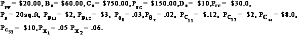
5. Numerical Examples For all models, let us assume, n = 2, a1= 9, a 2 = 10, Q01 = 10, Q02 =15, f1= 0.5 sq.ft. f2 = 0.8 sq.ft. The above non-linear programming problems (9), (15), (16) and (17) are solved by computer algorithm based on gradient search technique (Generalized Reduced Gradient method) for the following numerical data. 5 .1 Crisp Model: To illustrate the model (9), We assume
We first solved the multi-objective programming problem as a single objective problem subject to the space constraints using only one objective at a time and ignoring the rest objectives. Let Here, the values in the i-th column represent the optimum value of the i-th objective and the values of the order objectives at i) Fuzzy Programming Technique. From the above matrix P, the values of the bounds are With the above parametric values, the optimal values of model (15) are ii) Weighted Fuzzy Programming Technique. For the different values of
Table 1
iii) Goal Programming Technique: We solve the model (17) with the same parametric values of model (10) and
Table 2 ______________________________________________ 1 23.04 1.2 0.6 26.96 791.20 15.6 2 20.55 3.10 5.67 29.45 793.10 20.67 _____________________________________________ 5.2 Fuzzy Model: To illustrate the fuzzy model (28), we assume that all the crisp parametric values remain the same. In addition we take
6. Sensitivity Analysis Now, we perform some Sensitivity Analyses upon the profit, total cost, wastage costs, goals and warehouse space in fuzzy model due to the changes in the tolerance limits of
Table 3: Effect on PF, TC, FC and F due to incremental changes of ____________________________________________
_____________________________________________ 10 54.17 837.38 10.74 37.89 0.42 20 49.90 825.76 10.36 36.73 0.50 25 48.51 821.05 10.20 36.30 0.53 30 46.62 816.90 10.06 35.85 0.55 ______________________________________________________
Table 4: Effect on PF, TC, FC and F due to incremental changes of ___________________________________________
______________________________________________ 75 47.77 795.87 8.24 32.41 0.39 100 48.60 807.00 8.37 32.28 0.43 125 49.31 816.78 9.16 33.95 0.47 160 50.10 829.16 10.81 37.77 0.505 ______________________________________________
Table 5: Effect on PF, TC, FC and F due to incremental changes of __________________________________________
______________________________________________ 10 49.89 825.38 10.36 36.75 0.49 20 49.90 825.78 10.365 36.75 0.49 25 49.90 825.85 10.38 36.73 0.495 30 49.91 825.97 10.384 35.73 0.50 ______________________________________________
Table 6: Effect on PF, TC, FC and F due to incremental changes of _______________________________________________
_______________________________________________ 10 49.90 825.76 10.36 36.73 0.4949 20 49.90 825.76 10.36 36.76 0.4949 25 49.90 825.76 10.36 36.76 0.4949 30 49.91 825.76 10.36 36.76 0.4949
7. Conclusion From the above Tables - 3 to 6, it is observed that when
References
|
|||||
|
||||||