A New Sequential Non-Parametric Test for the Two Sample Problem
Keerthi M. Mathad*, I. D. Shetty
Department of Statistics, Karnatak University, Dharwad-580003, INDIA.
*Corresponding Address:
[email protected]
Abstract: A simple sequential non-parametric test for the two-sample problem is proposed. A method of deriving its ASN function for uniform and exponential distribution is given and their adequacy confirmed by simulation. The test is based on the normal approximation to the distribution of U-statistic. We also consider the small sample sensitivity. We restrict ourselves to the Lehmann alternative. The test is found to be performing well even for small sample size.
Keywords: Sequential; non-parametric; two-sample problem; average sample number; Lehmann alternative.
1. Introduction
Phatarfod and Sudbury (1988) considered a Wald-type test for the two-sample problem. Unlike in Bradley, Merchant and Wilcoxon (1966) they exploited the normal approximation to the Wilcoxon Mann-Whitney statistic. They first considered the Lehmann alternative and later on wider type of alternatives.
In this paper we consider a Wald-type test for the two-sample problem. We take 

 ,
,  . Here we wish to make a judgment between two new treatments and there is no prior preference involved. There would be a region of indifference
 , where, if the true situation was
 , it would not matter which of the two treatments was chosen. We propose the following Sequential test of strength
 . Observations are taken from the X and Y populations in pairs. At each stage, the U-statistic

Where 
 =Median of X1, X2, X3 and
  =Median of Y1,Y2, Y3
is calculated.
Sampling is continued as long as
 Where
Where  and
and 
And  or
or  is accepted according as the R.H.S or the L.H.S inequality is the first not satisfied.
2. Mean and Variance of the U-statistic when 
MEAN of U is given by 
 .
.
VARIANCE of U is given by
Var (U) =
Where,  = Covariance between the two kernels wherein cX observations and dY observations are in common between the two kernels.
Var (U)

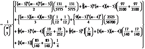 (2.1)
(2.1)
3. Mean and variance of the U-statistic when  and
and 
MEAN is given by 
VARIANCE of U is given by
Var(U)=
Where,  =Covariance between the two kernels wherein cX observations and dY observations are in common between the two kernels.
Var(U)
 (3.1)
(3.1)
Where,  ,
, ,
, ,
, ,
, ,
, ,
, ,
, ,
, are as defined earlier. Details are omitted for the sake of brevity.
4. The Sequential Non-Parametric Test
We have developed the SPRT based on the statistic U using the normal approximation to our statistic U when n is large for testing the simple hypothesis 
 Vs
Vs .
.
I.e. the continuation region at stage m is given by

Where  and
and 
5. The Average Sample Number
The sample size needed to reach a decision in a sequential or a multiple sampling plan is a random variable N, because at any stage of the experiment the decision to terminate the process depends on the results of the observations made earlier. The distribution of this random variable depends on the true distribution of the observations during the sampling process.
The ASN is given by
E  (n) = L (
 ) log B+ [1-L (
 )] log A/ E
  (z) where
  is the parameter
If E  (z) =0 then, E (n) =-logAlogB/E (z2)
Where E (z2) = ( 0-
0- 1)2/
1)2/ 2 i.e. E (n) = (-log A log B/(
 0-
0- 1)2)*
1)2)* 2
2
For this test the ASN function was obtained. To derive the ASN function, we note that the ASN function of our test is given by
E(N/K)=( L(K)log B+[1-L(K)]log A)/ E(z) Where, E(z)=
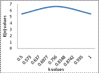
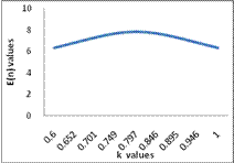
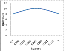
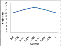
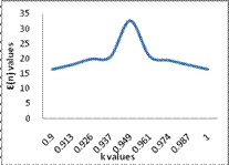
The following tables and graphs give the ASN for different values of k0
The values of ASN function for  and the corresponding graph.
Table 1

|

|

|

|
K |

|
-1 |
0.8935 |
0.04999 |
5.45 |
0.5 |
-0.75 |
0.8443 |
0.09901 |
5.81 |
0.573 |
-0.5 |
0.795 |
0.1866 |
6.19 |
0.637 |
0.25 |
0.7459 |
0.3238 |
6.49 |
0.6977 |
0 |
0.6967 |
0.5 |
6.62 |
0.756 |
0.25 |
0.6475 |
0.67609 |
6.49 |
0.8148 |
0.5 |
0.5983 |
0.81335 |
6.19 |
0.8742 |
0.75 |
0.5491 |
0.901 |
5.81 |
0.935 |
1 |
0.5 |
0.95 |
5.45 |
1 |
The values of ASN function for  and the corresponding graph
Table 2

|

|

|

|
K |

|
-1 |
0.8240 |
0.04999 |
6.34 |
0.6 |
-0.75 |
0.7835 |
0.09901 |
6.81 |
0.652 |
-0.5 |
0.743 |
0.1866 |
7.28 |
0.701 |
-0.25 |
0.7025 |
0.3238 |
7.66 |
0.749 |
0 |
0.662 |
0.5 |
7.81 |
0.797 |
0.25 |
0.6215 |
0.67609 |
7.66 |
0.846 |
0.5 |
0.581 |
0.81335 |
7.28 |
0.895 |
0.75 |
0.5405 |
0.901 |
6.81 |
0.946 |
1 |
0.5 |
0.95 |
6.34 |
1 |
The values of ASN function for  and the corresponding graph
Table 3

|

|

|

|
K |

|
-1 |
0.744 |
0.04999 |
8.07 |
0.7 |
-0.75 |
0.7135 |
0.09901 |
8.72 |
0.736 |
-0.5 |
0.6830 |
0.1866 |
9.38 |
0.773 |
-0.25 |
0.6525 |
0.3238 |
9.91 |
0.809 |
0 |
0.6220 |
0.5 |
10.109 |
0.845 |
0.25 |
0.5915 |
0.67609 |
9.91 |
0.883 |
0.5 |
0.5610 |
0.81335 |
9.38 |
0.921 |
0.75 |
0.5305 |
0.901 |
8.72 |
0.959 |
1 |
0.5 |
0.95 |
8.07 |
1 |
The values of ASN function for  and the corresponding graph
Table 4

|

|

|

|
K |

|
-1 |
0.6599 |
0.04999 |
11.98 |
0.80 |
-0.75 |
0.6391 |
0.09901 |
12.93 |
0.825 |
-0.5 |
0.6192 |
0.1866 |
13.94 |
0.848 |
-0.25 |
0.599 |
0.3238 |
14.61 |
0.873 |
0 |
0.579 |
0.5 |
15.33 |
0.898 |
0.25 |
0.559 |
0.67609 |
14.61 |
0.923 |
0.5 |
0.539 |
0.81335 |
13.94 |
0.949 |
0.75 |
0.519 |
0.901 |
12.93 |
0.975 |
1 |
0.5 |
0.95 |
11.98 |
1 |
The values of ASN function for  and the corresponding graph
Table 5

|

|

|

|
K |

|
-1 |
0.577 |
0.04999 |
16.38 |
0.90 |
-0.75 |
0.5673 |
0.09901 |
17.92 |
0.913 |
-0.5 |
0.557 |
0.1866 |
19.83 |
0.926 |
-0.25 |
0.5481 |
0.3238 |
20.67 |
0.937 |
0 |
0.5385 |
0.5 |
32.60 |
0.949 |
0.25 |
0.529 |
0.67609 |
20.77 |
0.961 |
0.5 |
0.5192 |
0.81335 |
19.39 |
0.974 |
0.75 |
0.5096 |
0.901 |
17.89 |
0.987 |
1 |
0.5 |
0.95 |
16.39 |
1 |
The test has greater ASN for the case K0=0.9
6. Average Sample Number for Uniform Distribution
We have compared our test with other tests for the same problem. We have considered two distributions, namely Uniform and Exponential distributions. We have found the mean and variance for the two distributions and later found the ASN function.
We have the uniform distribution


We have obtained the mean and variance of the statistic U under uniform distribution. The calculation is omitted for the sake of brevity.
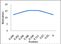
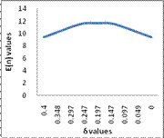
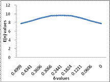
The ASN for different values of 
For 
Table 6

|

|

|

|

|
-1 |
0.3973 |
0.299 |
12.28 |
-0.75 |
0.4101 |
0.262 |
13.36 |
-0.5 |
0.4229 |
0.206 |
14.457 |
-0.25 |
0.4358 |
0.186 |
15.35 |
0 |
0.4487 |
0.148 |
15.4 |
0.25 |
0.4615 |
0.111 |
15.348 |
0.5 |
0.4743 |
0.0742 |
14.483 |
0.75 |
0.4871 |
0.0372 |
13.382 |
1 |
0.5 |
0 |
12.28 |

Table 7

|

|

|

|

|
-1 |
0.3642 |
0.4 |
9.41 |
-0.75 |
0.3812 |
0.348 |
10.199 |
-0.5 |
0.3982 |
0.297 |
11.006 |
-0.25 |
0.4151 |
0.247 |
11.63 |
0 |
0.4321 |
0.197 |
11.65 |
0.25 |
0.4491 |
0.147 |
11.63 |
0.5 |
0.4661 |
0.097 |
10.99 |
0.75 |
0.483 |
0.049 |
10.199 |
1 |
0.5 |
0 |
9.41 |
For 
Table 8

|

|

|

|

|
-1 |
0.3322 |
0.4999 |
7.77 |
-0.75 |
0.532 |
0.4341 |
8.39 |
-0.5 |
0.3742 |
0.3696 |
9.02 |
-0.25 |
0.3951 |
0.3066 |
9.51 |
0 |
0.4161 |
0.2441 |
9.62 |
0.25 |
0.4371 |
0.1824 |
9.51 |
0.5 |
0.4581 |
0.1211 |
9.01 |
0.75 |
0.479 |
0.0606 |
8.39 |
1 |
0.5 |
0 |
7.77 |
For 
Table 9

|

|

|

|

|
-1 |
0.3012 |
0.6 |
6.72 |
-0.75 |
0.3261 |
0.519 |
7.23 |
-0.5 |
0.3509 |
0.441 |
7.748 |
-0.25 |
0.3758 |
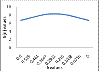
0.3647 |
8.167 |
0 |
0.4006 |
0.2901 |
8.25 |
0.25 |
0.4255 |
0.216 |
8.15 |
0.5 |
0.4503 |
0.1438 |
7.747 |
0.75 |
0.4752 |
0.0716 |
7.23 |
1 |
0.5 |
0 |
6.72 |
For 
Table 10

|

|

|

|

|
-1 |
0.2715 |
0.7 |
6.00 |
-0.75 |
0.3 |
0.6039 |
6.434 |
-0.5 |
0.3286 |
0.5113 |
6.87 |
-0.25 |
0.3572 |
0.4217 |
7.227 |
0 |
0.3858 |
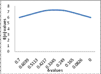
0.3345 |
7.31 |
0.25 |
0.4143 |
0.249 |
7.225 |
0.5 |
0.4429 |
0.165 |
6.87 |
0.75 |
0.4714 |
0.0826 |
6.434 |
1 |
0.5 |
0 |
6.00 |
7. Average Sample Number for Exponential Distribution
We now consider the exponential distribution we have found the mean and variance for the distribution and later found the ASN function.
We have the exponential distribution


We have obtained the mean and variance of the statistic U under exponential distribution. The calculation is omitted for the sake of brevity.
The ASN for different values of δ
For 
Table 11

|

|

|

|

|
-1 |
0.3313 |
0.3 |
7.738 |
-0.75 |
0.3524 |
0.258 |
8.352 |
-0.5 |
0.3735 |
0.2188 |
8.977 |
-0.25 |
0.3946 |
0.1804 |
9.48 |
0 |
0.4156 |
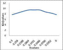
0.1431 |
9.5 |
0.25 |
0.4367 |
0.1066 |
9.48 |
0.5 |
0.4578 |
0.0706 |
8.976 |
0.75 |
0.4789 |
0.0352 |
8.352 |
1 |
0.5 |
0 |
7.738 |
For 
Table 12

|

|

|

|

|
-1 |
0.2839 |
0.4 |
6.28 |
-0.75 |
0.3109 |
0.3417 |
6.739 |
-0.5 |
0.3379 |
0.2868 |
7.206 |
-0.25 |
0.3649 |
0.2349 |
7.577 |
0 |
0.3919 |
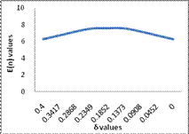
0.1858 |
7.62 |
0.25 |
0.4189 |
0.1373 |
7.587 |
0.5 |
0.4459 |
0.0908 |
7.212 |
0.75 |
0.4729 |
0.0452 |
6.742 |
1 |
0.5 |
0 |
6.28 |
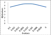
For 
Table 13

|

|

|

|

|
-1 |
0.2418 |
0.5 |
5.46 |
-0.75 |
0.2741 |
0.422 |
5.837 |
-0.5 |
0.3064 |
0.3511 |
6.218 |
-0.25 |
0.3386 |
0.2855 |
6.518 |
0 |
0.3709 |
0.2237 |
6.55 |
0.25 |
0.4032 |
0.1650 |
6.517 |
0.5 |
0.4355 |
0.1086 |
6.214 |
0.75 |
0.4677 |
0.0539 |
5.837 |
1 |
0.5 |
0 |
5.46 |
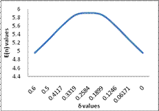
For 
Table 14

|

|

|

|

|
-1 |
0.2049 |
0.6 |
4.96 |
-0.75 |
0.2418 |
0.5 |
5.27 |
-0.5 |
0.2787 |
0.4117 |
5.598 |
-0.25 |
0.3156 |
0.3319 |
5.86 |
0 |
0.3525 |
0.2584 |
5.91 |
0.25 |
0.3893 |
0.1899 |
5.86 |
0.5 |
0.4262 |
0.1246 |
5.598 |
0.75 |
0.4631 |
0.06171 |
5.27 |
1 |
0.5 |
0 |
4.96 |
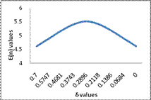
For 
Table 15

|

|

|

|

|
-1 |
0.1729 |
0.7 |
4.62 |
-0.75 |
0.2138 |
0.5747 |
4.901 |
-0.5 |
0.2547 |
0.4681 |
5.186 |
-0.25 |
0.2956 |
0.3743 |
5.415 |
0 |
0.3365 |
0.2896 |
5.52 |
0.25 |
0.3773 |
0.2118 |
5.414 |
0.5 |
0.4182 |
0.1386 |
5.185 |
0.75 |
0.4591 |
0.0684 |
4.901 |
1 |
0.5 |
0 |
4.62 |
Conclusions
ASN for different values of 
For  |
For  |
For  |
For  |
For  |
Uniform |
Exponential |
Uniform |
Exponential |
Uniform |
Exponential |
Uniform |
Exponential |
Uniform |
Exponential |
12.28 |
7.73 |
9.41 |
6.28 |
7.77 |
5.46 |
6.72 |
4.96 |
6.00 |
4.62 |
13.36 |
8.35 |
10.19 |
6.73 |
8.39 |
5.83 |
7.23 |
5.27 |
6.43 |
4.90 |
14.45 |
8.97 |
11.006 |
7.206 |
9.02 |
6.21 |
7.74 |
5.59 |
6.87 |
5.18 |
15.35 |
9.48 |
11.63 |
7.57 |
9.51 |
6.51 |
8.16 |
5.86 |
7.22 |
5.41 |
15.19 |
9.32 |
11.44 |
7.46 |
9.36 |
6.43 |
8.03 |
5.77 |
7.11 |
5.34 |
15.34 |
9.48 |
11.63 |
7.58 |
9.51 |
6.51 |
8.15 |
5.86 |
7.22 |
5.41 |
14.48 |
8.97 |
10.99 |
7.21 |
9.01 |
6.21 |
7.74 |
5.59 |
6.87 |
5.18 |
13.38 |
8.35 |
10.19 |
6.74 |
8.39 |
5.83 |
7.23 |
5.27 |
6.43 |
4.90 |
12.28 |
7.73 |
9.41 |
6.28 |
7.77 |
5.46 |
6.72 |
4.96 |
6.00 |
4.62 |
The results appear in the table. It is seen that for the exponential distribution ASN behaves better than the uniform in having smaller error probabilities and lower ASN, the ASN in general being less than half the fixed sample size for the test of the difference of two means from normal populations with equal known variance.
References
- Abraham Wald (1947). Sequential Analysis, New York: John Wiley and Sons, Inc. Chapman and Hall, Ltd, London.
- Bradley, R.A, Merchant, S.D. and Wilcoxon, F. (1966). Sequential rank tests II modified two sample procedures. Technometrics, 8, 615-623.
- Cox. D.R. (1952). Sequential tests for composite hypotheses Proceedings of the Cambridge Philosophical society, 48, 290-299.
- Ghosh, B.K.(1970). Sequential tests of Statistical Hypotheses. Reading, M.A; Addison-Wesley.
- Gibbons. J.D and Subhabrato Chakraborti. (1992). Non-parametric Statistical Inference. Marcel Dekker, Inc. New York.
- H.B. Mann and D.R. Whitney. (1947). on a test of whether one of two random variables is stochastically larger than the other. Ann. Math. Statist, 18, 50-60.
- H.F. Dodge and H.G. Romig. (1929). A Method of Sampling Inspection, The Bell System Technical Journal, Vol.8, pp.613-631.
- H.Scheffe. (1943). Statistical Inference in the Nonparametric case. Ann. Math. Statist. 14, 305-32.
- Hoeffding, W. (1948). A class of statistics with asymptotic normal distribution, Ann. Math. Statist, 19, 293-325.
- Lai, T.L. (1975). On Chernoff-Savage Statistics and Sequential rank tests. Ann. Statist. 3, 825-845.
- Lehmann, E.L. (1951). Consistency and Unbiasedness for certain non-parametric tests, Ann. Math. Statistics, 22, 165-179.
- Lehmann, E.L. (1975). Non-parametric, San Francisco: Holden-Day.
- Mathisen, H.C. (1943). A method of testing the hypothesis that two samples are from the same population. Ann. Math. Statistics, 14, 188-194.
- Miller, R. G. Jr. (1969). Sequential signed-rank test. J. Amer. Statist. Assoc. 65, 1554-1561.
- Miller, R. G. Jr. (1972). Sequential rank tests-one sample case. Proc. Sixth Berkeley Symp.Math Statist.Prob. 1, 97-108.
- Phatarfod, R.M. and Aidan Sudbury. (1988). A simple Sequential Wilcoxon test. Austral. J. Statist, 30(1), 93-106.
- Pitman, E. J.G. (1948). Notes on non-parametric statistical inference. Columbia University.
- Randles, R. H. and Wolfe, D. A. (1979). Introduction to the Theory of Non parametric Statistics, Wiley, New York.
- Savage, I. R, and Sethuraman, J. (1966). Stopping time of a rank order sequential probability ratio test based on Lehman alternatives. AMS 37, 1154-1160.
- Shetty, I.D, and Z. Govindarajalu. (1988). A two-sample test for location, Comm. in Statistics-Theory and Methods, 17, 2389- 2401.
- Shetty, I.D. and Bhat, S.V. (1993). Some Competitors of Mood’s Median test for the location alternative, Journal of Karnataka University-Science, 37, 11, 138-146.
- Wilcoxon, F, Rhodes, L.J. and Bradley, R.A. (1963). Two Sequential two-sample grouped rank tests with applications to screening experiments, Biometrics, 19, 58-84.


 (2.1)
(2.1)


 (3.1)
(3.1)